2026 Methods
The Forward-Forward Algorithm: Learning Without Going (Fully) Backward
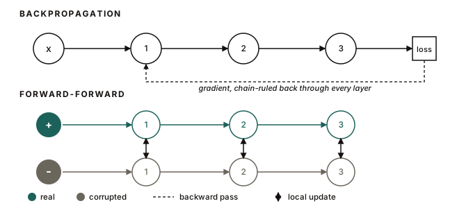
Backpropagation is the algorithm behind most of the last decade of deep learning. It’s also, in Hinton’s own words, something that “as a model of how cortex learns… remains implausible despite considerable effort to invent ways in which it could be implemented by real neurons.” It needs every intermediate activation kept around until an error signal reaches the output, and then that signal has to travel backward through the exact same weights, layer by layer, in reverse. Real neurons don’t obviously do that, and it doesn’t map cleanly onto analogue or neuromorphic hardware either. In late 2022, Hinton published this paper proposing something different: the Forward-Forward algorithm. No backward pass. Two forward passes instead.
The core idea
Every layer in a Forward-Forward network trains on its own, using only its own input and its own output. There’s no end-to-end loss, no computational graph spanning the whole network, and no gradient that ever has to travel from a later layer back to an earlier one.
To train a layer, you show it two kinds of data:
- Positive data: real examples, the kind you want the layer to respond strongly to.
- Negative data: corrupted or mismatched examples, the kind you want it to respond weakly to.
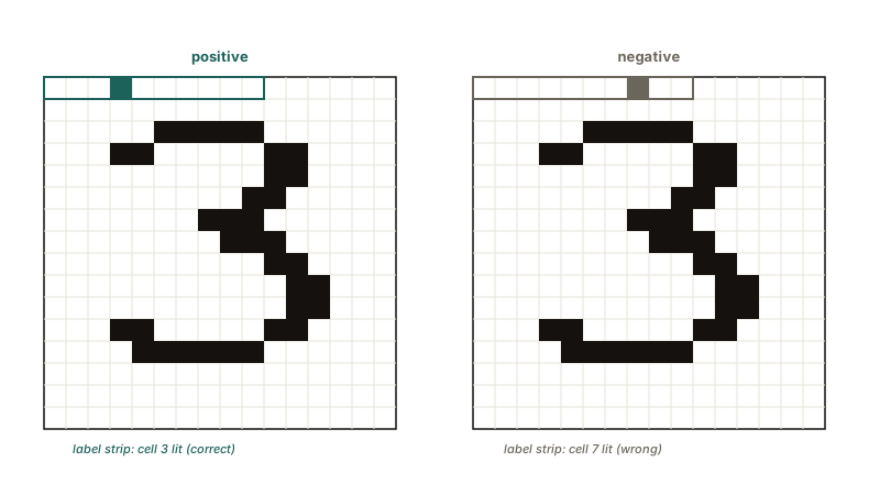
Each layer computes a single number from its own activity, called goodness: just the mean squared activity of its output units. Training nudges that layer’s weights, and only that layer’s weights, to push goodness up for positive data and down for negative data. That’s about as simple as logistic regression gets, with the goodness score standing in for the prediction. The gradient only ever touches that one layer’s own weights.
One more piece worth knowing about: before a layer’s output moves on to the next layer, it gets
length-normalised, divided by its own norm. Here’s why that matters, in plain arithmetic:
goodness is Σ yᵢ², the sum of the squared activities in the output vector y. Multiply every
entry of y by some constant k, and goodness gets multiplied by k². So a layer could raise
its goodness for free just by scaling everything up, without learning anything about which units
should actually be active. Dividing y by its own norm, ‖y‖ = √(Σ yᵢ²), kills that shortcut:
whatever the raw activity was, the vector handed to the next layer always has length 1. All that
survives is the ratio between units, yᵢ / ‖y‖, not their overall scale.
Where the negative data comes from
For supervised classification, Hinton’s trick (borrowed here for the notebook below) is to bake the label directly into the input. Overlay a one-hot label onto a handful of pixels (the corner of an MNIST digit, say): the positive example gets the correct label, the negative one gets a wrong label. A network that gets good at telling these apart is, along the way, learning to recognise digits. For unsupervised settings, Hinton generates negatives by blending two unrelated images together with a random mask and training the network to prefer the un-blended original, no labels involved at all.
At inference time there’s no classifier head to read off either, since that would need a gradient travelling back from a loss into all the feature layers, exactly what we’ve been avoiding. Instead you try overlaying every candidate label onto the test image, run each version through the network, and take whichever label produced the highest total goodness. It costs one forward pass per class, but it’s simple: it’s exactly what the network was already trained to compute.
Does it actually work?
The best way I know to convince myself an idea like this is real, rather than just a nice
sketch, is to implement it with nothing to hide behind: no autograd, no framework computing
gradients for me. So I wrote a NumPy-only Forward-Forward network,
trained on the small digits dataset from scikit-learn (1,797 8×8 handwritten digits, not
MNIST, so the whole thing trains in well under a minute on a laptop CPU).
Two hidden layers of 256 units, trained one at a time, 500 epochs each, using the labels-in-the-corner trick above for negative data. The gif below is the notebook’s own output: two stacked panels, one per layer, playing in lockstep by snapshot index rather than wall-clock time (layer 2 only starts once layer 1 is done, so “same frame” means “same point in that layer’s own schedule”). At epoch 0 both panels show positive and negative piled on top of each other: a freshly initialised layer has no opinion about anything yet. By the end each has cleanly split either side of the threshold, and that separation is the entire training signal; there’s nothing else driving these weights.
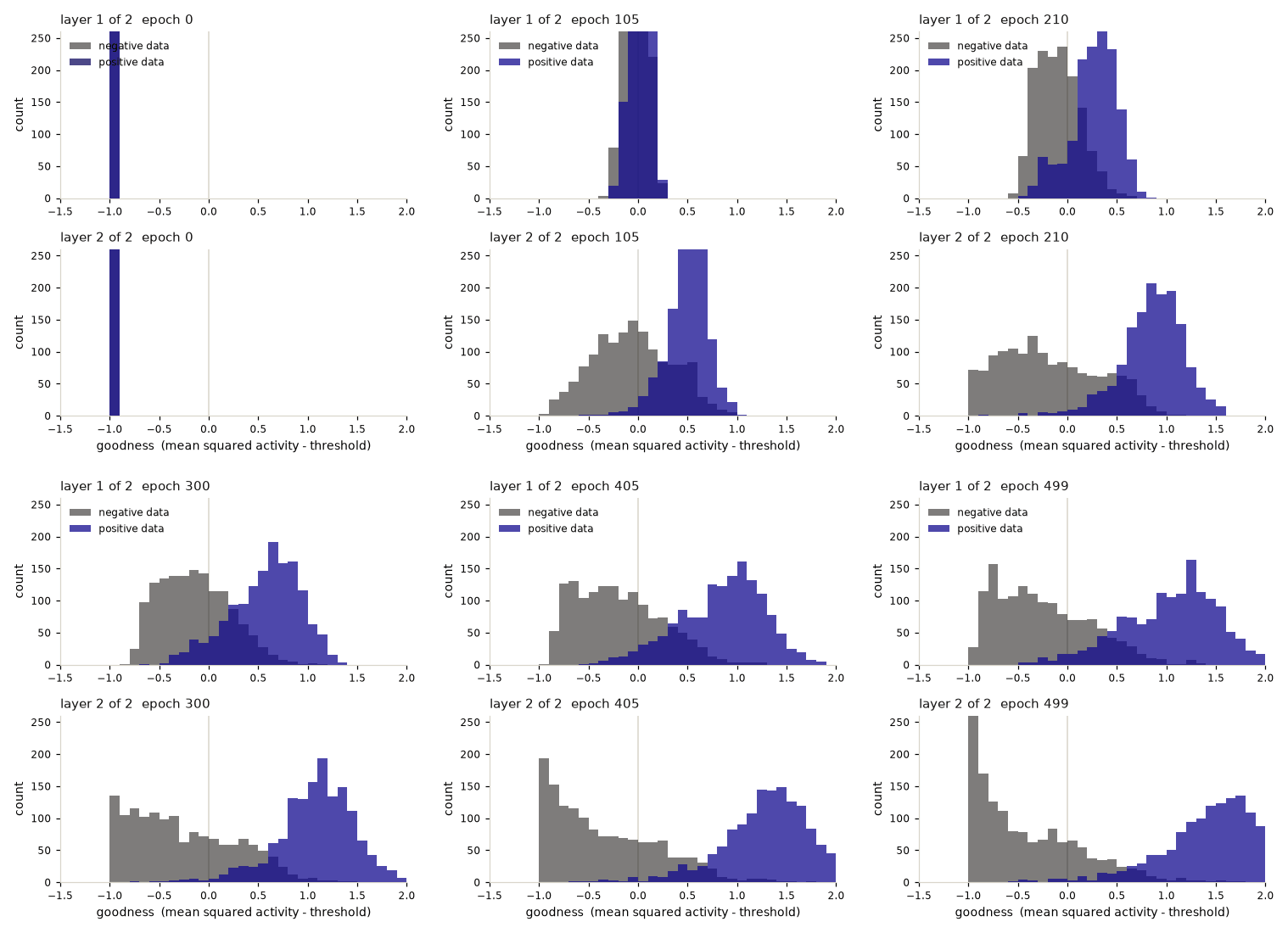
With no output layer, no cross-entropy loss, and no gradient ever crossing a layer boundary, the “try every label and keep the highest goodness” classifier gets 86.4% test accuracy on held-out digits, against a 10% chance baseline. It never once computed a loss gradient with respect to anything other than its own layer’s weights, and it still learned to tell nines from fours.
The notebook has the full implementation, including the per-layer update rule spelled out as plain array arithmetic, and it regenerates the gif above from scratch when you run it.
Does it work for a CNN too?
Everything above used dense layers, with the label overlaid directly onto a handful of pixels. A convolutional layer can’t overwrite “a few pixels” like that, since the input has to stay a 2D image, so the label gets a different encoding: one constant-valued plane per class, stacked alongside the image. The positive example fills in its true class’s plane, the negative example fills in a wrong class’s plane, and every other plane stays at zero. Same layer, same goodness, same local update, just a 3x3 convolution instead of a dense one.
I tried a simpler version first, a single channel encoding the class index directly rather than ten one-hot planes. It trains, just much more slowly, probably because ten planes give the kernel ten independent things to key on, where one ordinal channel asks it to learn a subtler distinction, between class 4 and class 5, say. I kept the one-hot version for the result below and left the single-channel one as a note in the notebook.
Two lessons came out of getting the one-hot version to actually train.
First, the label plane can’t be constant over the whole image, the way Hinton describes it: that barely trained at all, stuck at chance for hundreds of epochs. A convolution applies the same kernel everywhere, so a label signal that’s identical everywhere gives the kernel nothing local to key on. Confining it to a small corner patch fixes that.
Second, what actually decides accuracy at higher resolution is training-set size, not patch geometry. The 16x16 run only had 250 images to learn from, a fraction of the 8x8 run’s full set, and that’s the more binding constraint. It also converges best trained as one single batch, all the available samples on every epoch, rather than split into mini-batches: goodness is a much noisier signal to learn from when a batch only sees a handful of examples at a time.
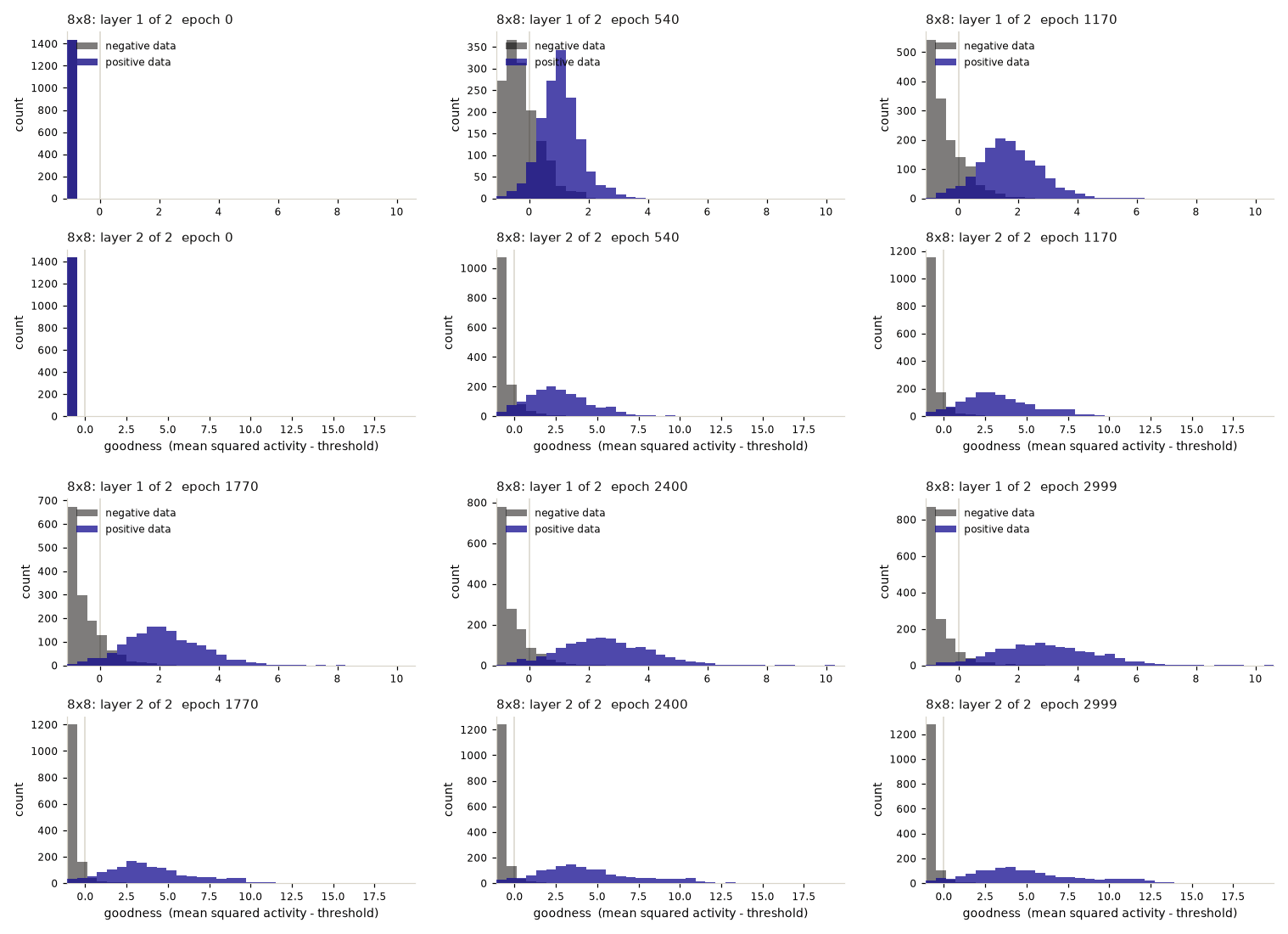
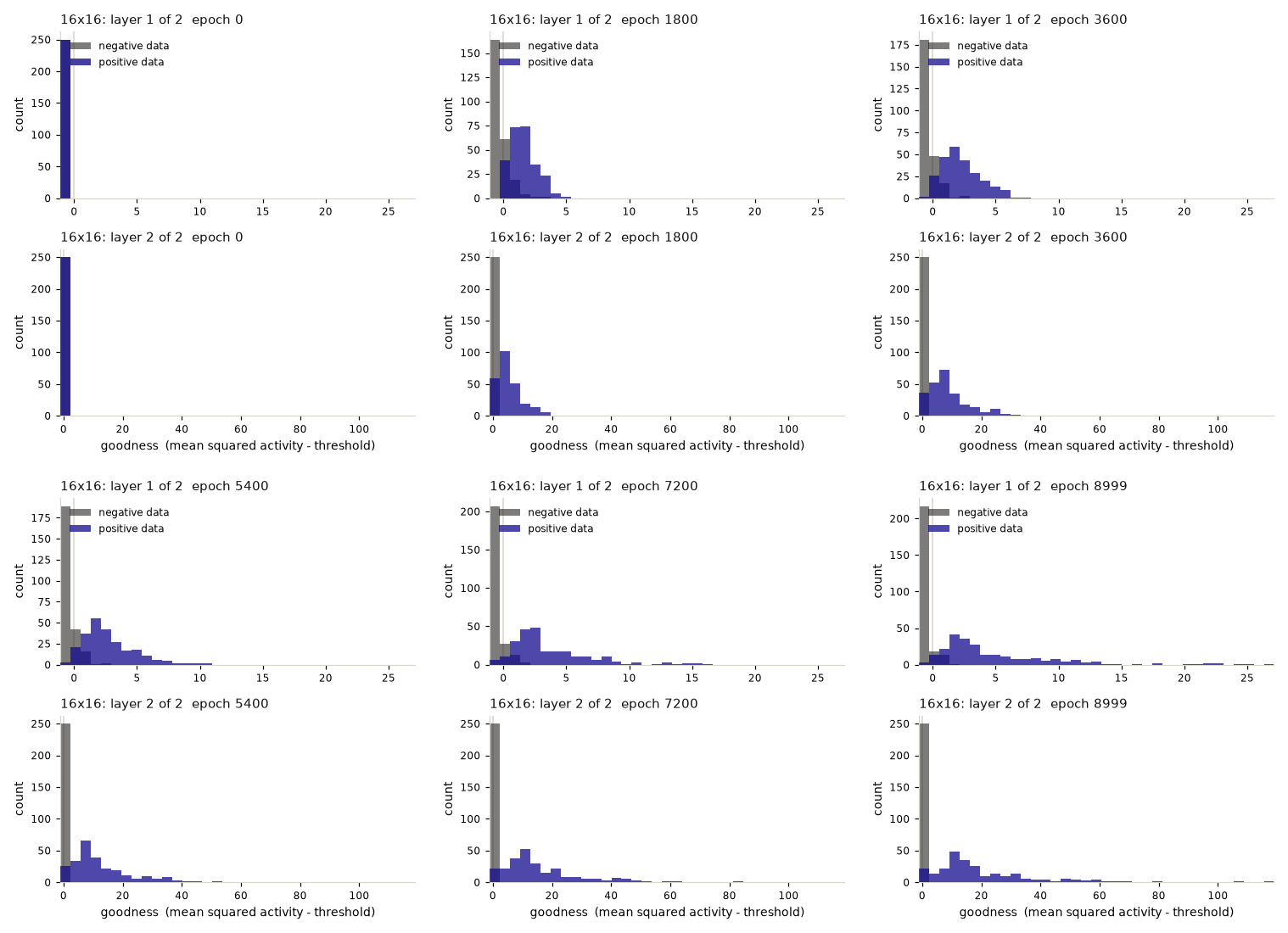
Two convolutional layers, scored the honest way (excluding layer 1’s goodness from the vote, since layer 1 is the one that saw the label directly), converge cleanly at both native 8x8 resolution and, upsampled and trained on a smaller subsample with three times the epoch budget, at 16x16 too. I didn’t tune either run beyond getting it to converge (no layer norm, no batch norm, no learning-rate schedule), so there’s room to push further with the usual training tricks. The notebook has the exact numbers and is the place to go try that.
Our extensions
Forward-Forward isn’t a finished or published piece of work: Hinton put it on arXiv in December 2022, called it “preliminary investigations,” and it’s never been peer reviewed. It’s also not yet a practical replacement for backprop, being slower per epoch and untested past modestly sized networks. What it gives up is the requirement that the whole network be differentiable end to end, which would let layers train asynchronously without a global backward pass, and the need to store activations for a backward pass at all, relevant for spiking networks or analogue chips. What it keeps is an explicit, differentiable objective for every layer, unlike the hand-tuned Hebbian rules that biologically-plausible-learning research relied on before it. The goodness function itself, a single number for how much an input resembles what a network was trained on, computed with no label and no reconstruction target, maps onto anomaly detection: deciding whether a scan matches a model’s training distribution or looks rarer and unlabelled. That’s the basis for two further papers extending the idea.
Every hyperparameter I hand-tuned for the toy network above (how wide each layer is, where the goodness threshold sits) was, in Resource-Efficient Medical Image Analysis with Self-adapting Forward-Forward Networks (Müller & Kainz, MLMI 2024), something I made the network set for itself instead. Medical imaging datasets are exactly the setting where you can’t afford to grid-search architecture and threshold per task: cohorts are small, and there usually isn’t a spare validation set large enough to tune on safely, so the network grows or prunes its own layers and re-centres its own threshold as it trains, rather than inheriting values picked for MNIST. It’s the same local, layer-at-a-time update this whole post has been about, just no longer trusting me to have picked good defaults for it.
The second paper, Self-Adaptive Forward-Forward Network for Anomaly Detection and Medical Image Analysis (Müller, Baugh & Kainz, Frontiers in Radiology, 2026), is where the “does this feel familiar” reading of goodness stops being a metaphor and becomes the whole point. Goodness becomes directly a novelty score, trained self-supervised on normal anatomy alone: positive examples are real scans, negative examples are synthetic corruptions generated from those same scans, so no labelled anomalies are needed anywhere in training. Run an unseen scan through the network and a low goodness (the same quantity that was pushed above threshold for positive, real examples during training) is itself evidence that something in the image doesn’t belong. No separate anomaly-detection head, no reconstruction error from an autoencoder, nothing extra bolted on. The classifier described earlier in this post tries every label and keeps the best score; an anomaly detector just asks whether the best score it can find is still low, and that’s the whole model.
Neither paper claims backprop has some fundamental flaw that Forward-Forward fixes: on identical data, a well-tuned, normally trained network is still hard to beat outright. What our extensions lean on instead is that each layer’s update stays its own small, local, adaptable thing, not bound to one global objective, so it’s easy to ask it to adapt to a dataset a hundred times smaller than MNIST, or to answer a different question entirely, not “which class is this” but “have I seen anything like this before,” without redesigning the network around a new loss.